Machine Learning Isn't Magic; It's Just Optimization

Rather than listing machine learning models and techniques, I want to start from first principles and build up the idea of machine learning. Some problems seem intractable in computer science, like programmatically determining whether an image shows a dog. If you knew nothing about machine learning, it'd be hard to imagine where you'd even start.

On the other hand, there are far simpler problems we do know how to solve. So it makes sense to start with a simple problem we can solve and gradually make it harder until it resembles the difficult problem we care about.

Optimizing a Quadratic Polynomial

Suppose we're running a business and want to maximize our revenue from a product. We notice that if we price the product at dollars, we can sell units. Now we want to find the value of that maximizes our revenue .

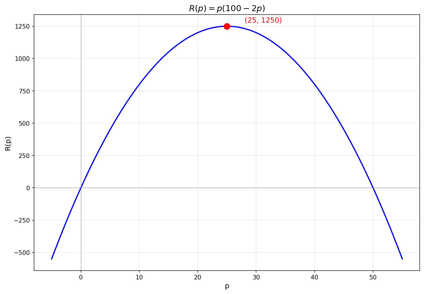
There are multiple approaches we could use to maximize a simple quadratic polynomial. One way is to complete the square and rewrite as , which is maximized at since the squared term with a negative coefficient is always nonpositive.

A more general-purpose approach is to find the critical points by setting the derivative to , then choose the one that maximizes the function. In this case, is the only critical point.

A still more general approach, when we can't solve , is to start at a random point and iteratively move in the direction that increases the function. Recall the limit definition of the derivative: . Rearranging, this tells us that for a small step , the function changes by approximately . So if , a positive step increases , and if , a negative step increases .

The simplest approach is to just use the sign of the derivative: , where is a fixed step size. Starting at with :

Each step moves by a fixed amount in the direction of increasing . With , we land exactly on after steps; in practice, we'd stop when is near zero or when the updates begin to flip signs.

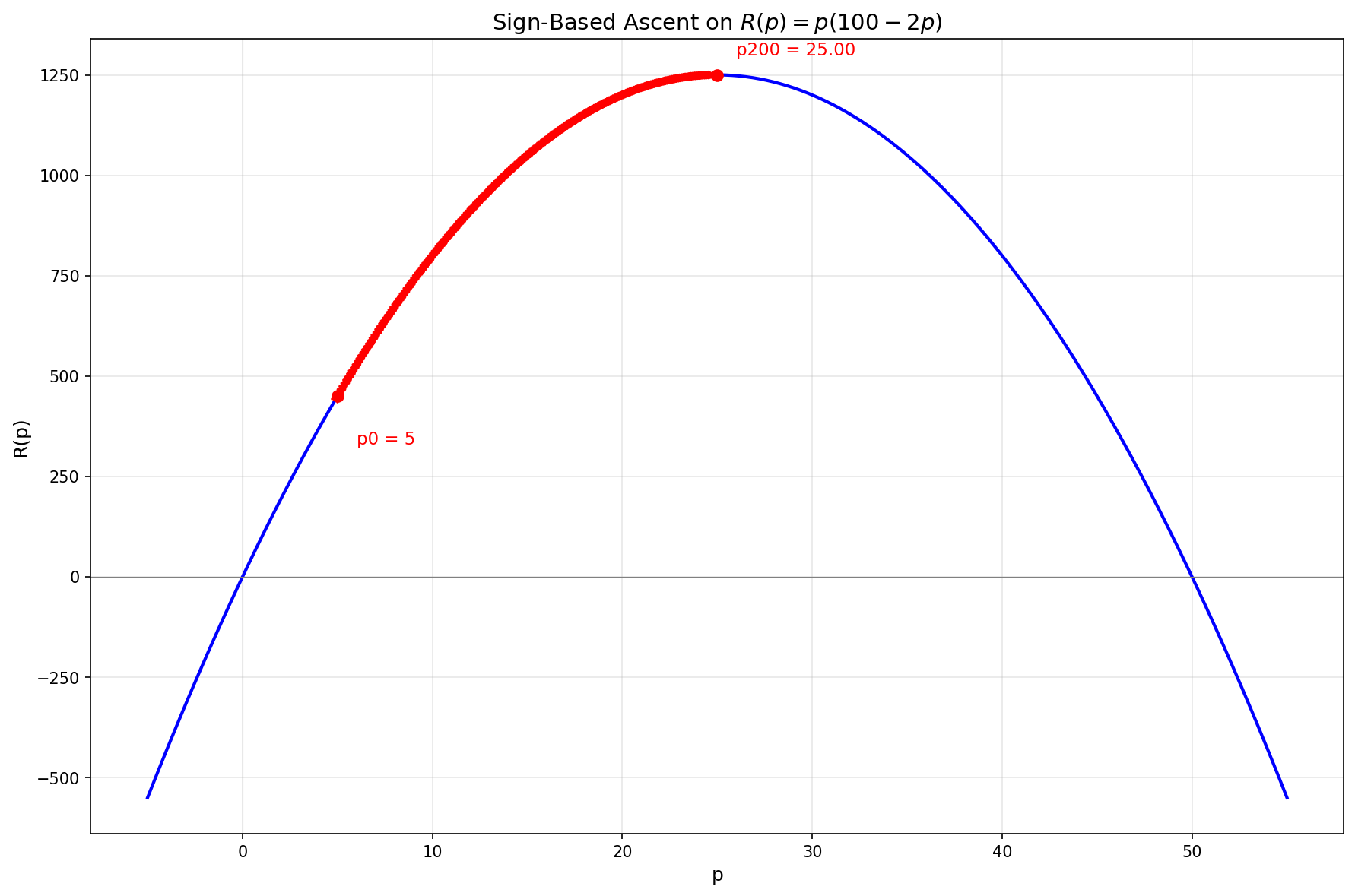
This works, but the fixed step size is a limitation. If the step is too large, we might overshoot the maximum and oscillate around it. If it's too small, convergence is slow. We can do better by also using the magnitude of the derivative: taking larger steps when we're far from the peak (where the slope is steep), and smaller steps as we approach it (where the slope flattens).

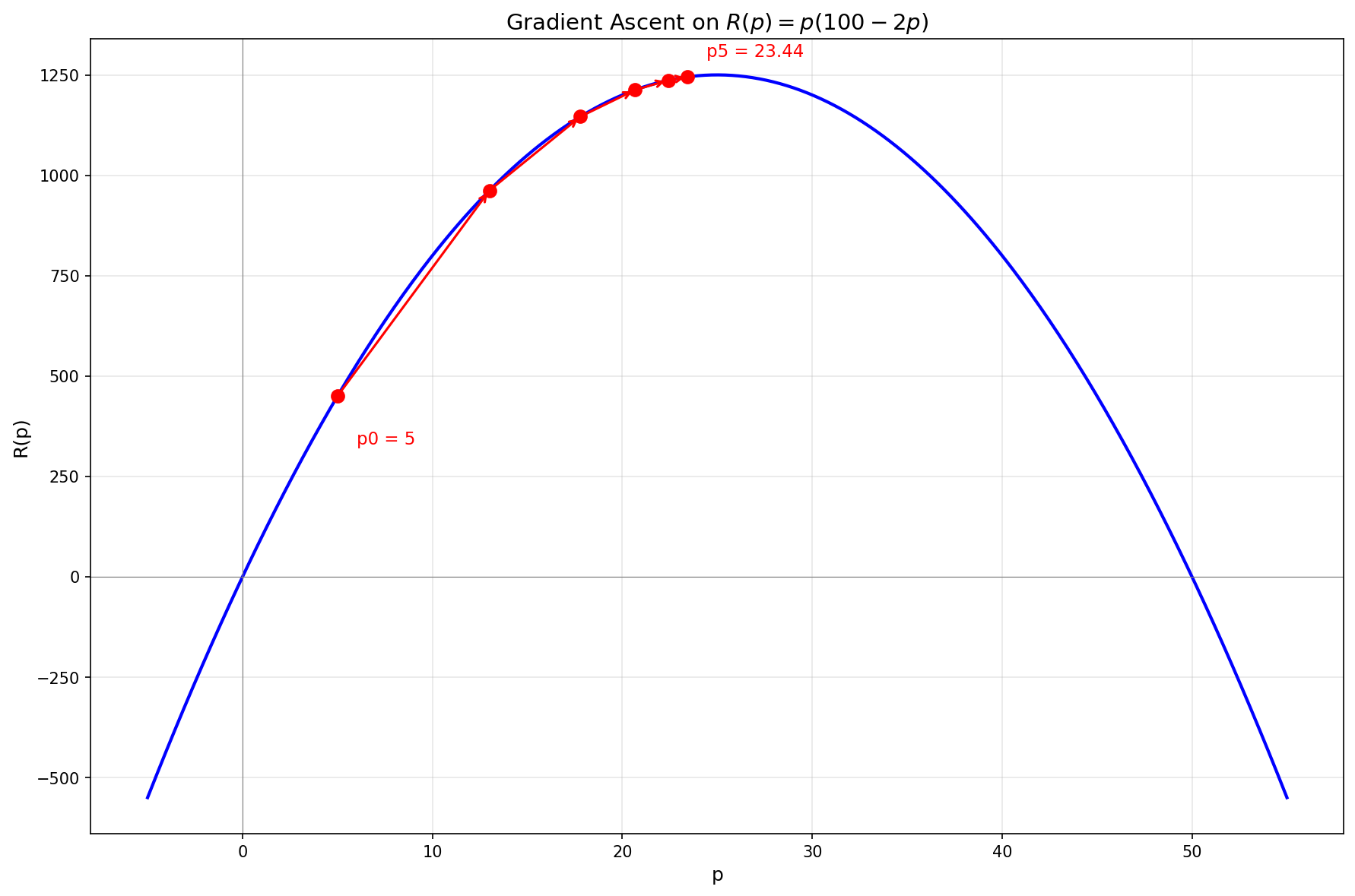
This gives us gradient ascent with the update rule , where controls the step size. Starting at with :

Now the steps naturally get smaller as we approach the peak, allowing for both fast initial progress and precise convergence.

Now let's move on to a more complex function.

Optimizing a Single-Variable Function

The previous example was a quadratic, where we could solve analytically to find the critical point. But what if the derivative equation has no closed-form solution?

Consider . Setting the derivative to zero gives , which has no simple closed-form solution. This is where gradient descent becomes essential rather than just convenient.

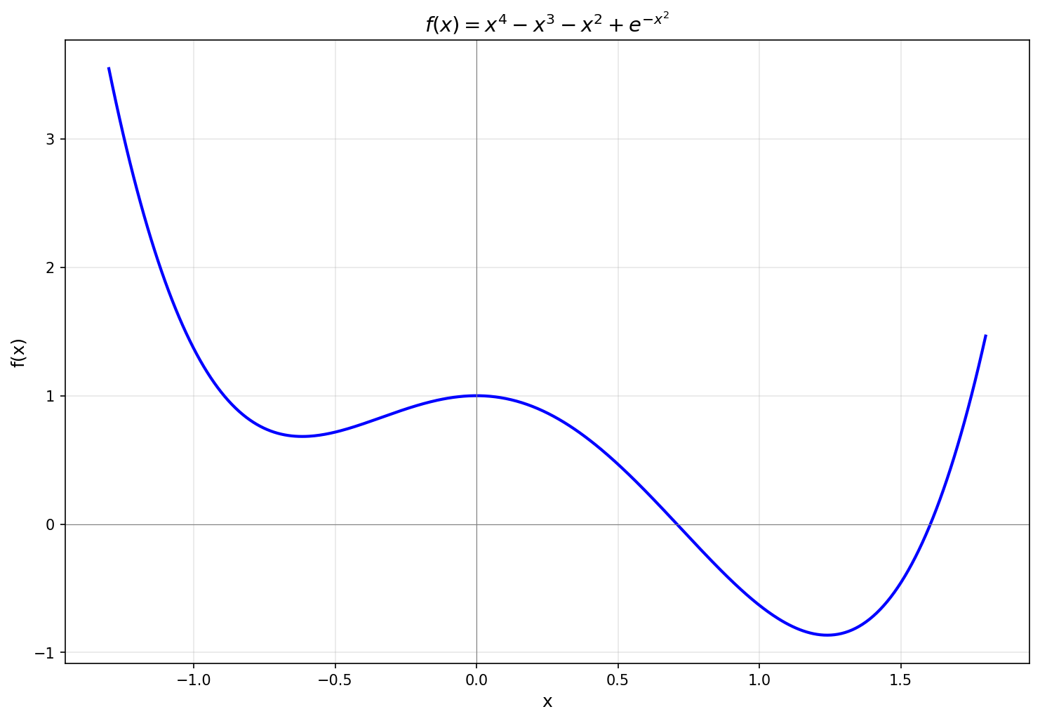
This function has two local minima, one near and a deeper one near . Since we're minimizing instead of maximizing, the update rule becomes (note the minus sign). Starting from with :

After a few more steps, converges to the minimum at .

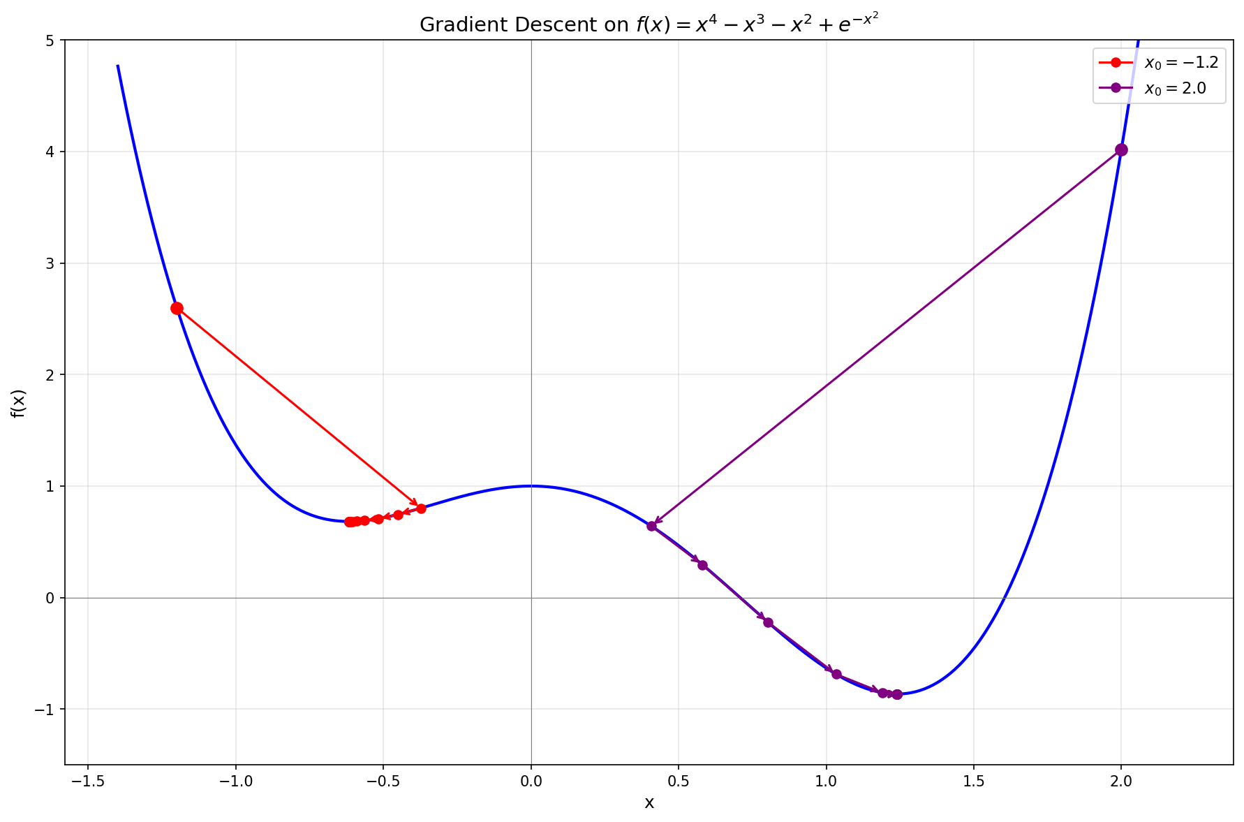
The plot shows two different starting points. Starting from leads to the deeper minimum on the right, while starting from leads to the shallower minimum on the left. The starting point determines which minimum we find, since gradient descent finds a local minimum, not necessarily the global one.

Optimizing a Two-Variable Function

Now let's add another variable. Consider , which has a minimum at the origin.

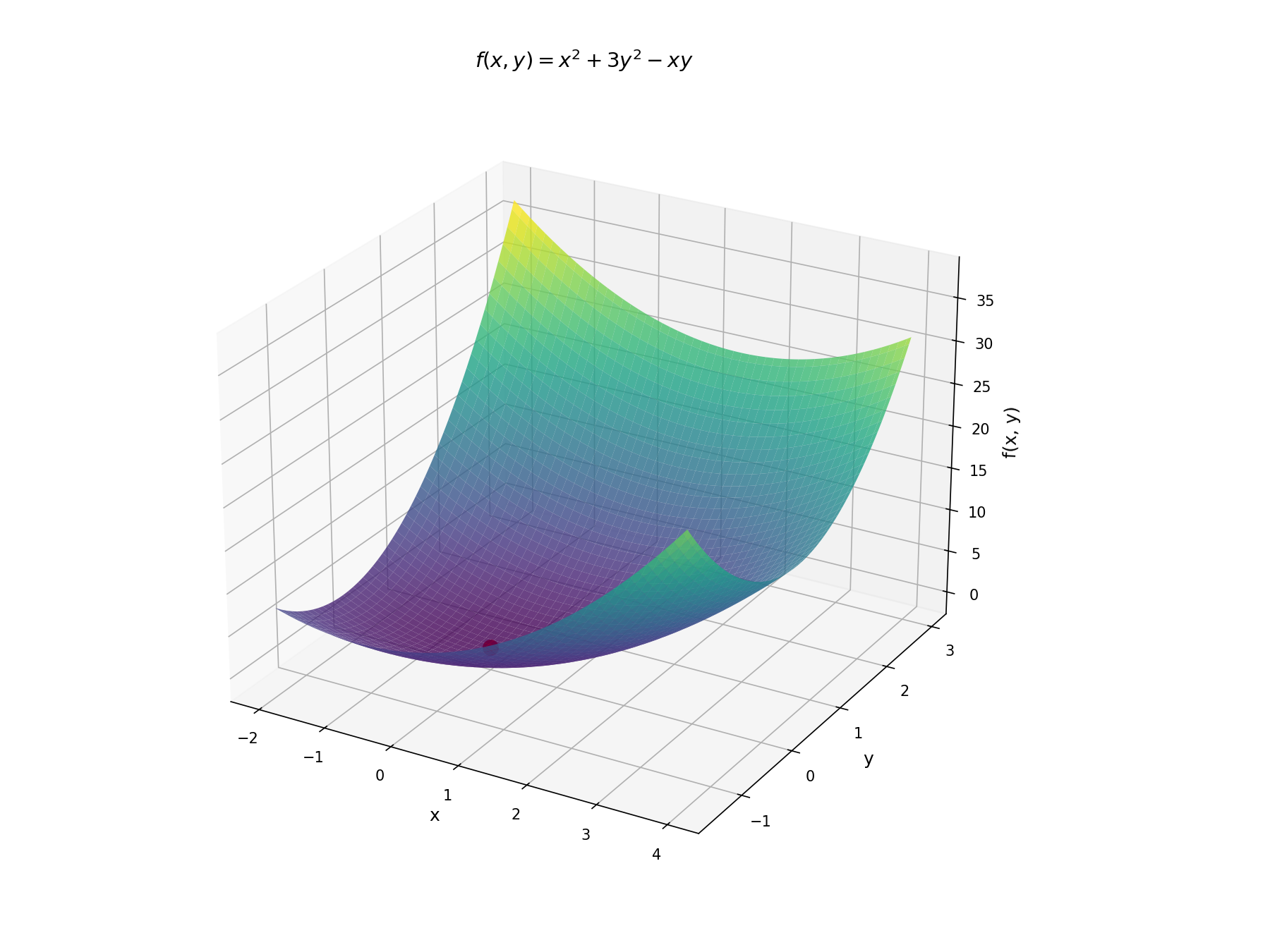
In the single-variable case, we minimized by changing in the direction that decreased . With two variables, the same idea applies in both coordinates: how should we change (holding fixed) to decrease , and how should we change (holding fixed) to decrease ? A small step changes the function by the sum of the partial contributions:

Together, those partial derivatives form a vector called the gradient:

The gradient points in the direction of increasing , so for small enough we subtract it to descend. This is the same idea as the single-variable update , where we replace the scalar derivative with a vector and take a proportional step in parameter space. The update rule is structurally identical to before:

Starting from with :

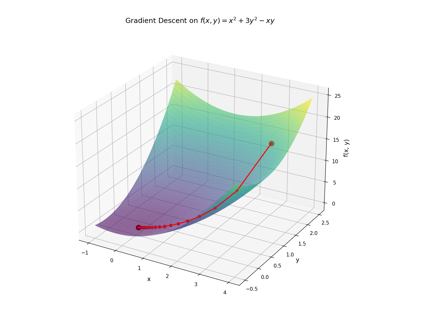
Notice that the path doesn't head straight toward the minimum; it curves because the function is steeper in the direction. But the algorithm doesn't need to know this; it just follows the gradient downhill at each step.

Nothing fundamentally changed from the single-variable case. We're still computing a derivative and stepping opposite to it. The only difference is that our derivative is now a vector.

In one dimension, there are only two directions to move, and only one decreases the function locally. In two dimensions, there are infinitely many descent directions, so in principle there are many update rules we could use, such as changing one variable at a time. So what's special about the gradient vector?

If we fix the length of a small update step , the change is , and by Cauchy-Schwarz this is most negative when points opposite . So the steepest local decrease direction is . A standard update rule is therefore , where sets the step size. Although we don't have to follow this direction, it explains why descending along the gradient is a principled default.

Creating a Simple Model

Now that we have some tools, let's go back to the original problem of programmatically identifying whether an image shows a dog. Mathematically, we want to find a function such that and .

What kind of function could be? It could involve arbitrarily complex expressions, and we have no reason to expect it to take any particular form. The universal approximation theorem gives us a way forward. Under mild conditions, a neural network with enough parameters can approximate any function arbitrarily well. This reduces the problem from searching over all possible mathematical expressions to finding the right parameters for a neural network .

Now we need to determine what parameters give us the function we want. We already know how to minimize functions with gradient descent, so we need to turn "find parameters that make accurate" into "minimize some function of ."

The function on its own has no notion of being minimized or maximized. But we can define a new objective function that measures how wrong is. Suppose we had access to every possible dog image and every possible non-dog image. We want to output for each dog image and for everything else, so we can measure the total error as

Every term in this sum is zero when the prediction is correct and positive otherwise, so is minimized precisely when correctly classifies every image. This isn't the only function we could choose though. Instead of squaring, we could raise it to the fourth power, or take the absolute value, and it would still be minimized when correctly classifies every image. Squaring is a nice choice because its derivative is smooth and easy to compute.

Of course, this objective is intractable in practice since we can't enumerate every possible image. Instead, we collect a training dataset of labeled images, a representative sample of the full distribution. If we let denote the label of the th training image ( for dog, otherwise), we replace the sum over all images with a sum over just our dataset:

This is called the loss function. It takes the neural network's parameters and returns a single number measuring how poorly the model performs on the training data. Minimizing it is structurally the same problem as the ones above. We compute , step opposite to it, and repeat. The parameters play the same role as or did earlier; the only difference is that there may be millions of them instead of one or two.

---

The idea behind machine learning with neural networks follows directly from optimization. We define a function that measures error, and minimize it with gradient descent. There's no new mathematical machinery beyond what we've already built up.

Of course, there are plenty of open questions I haven't addressed here. How do we make a model generalize well with limited training data? How do we make training work well when the loss landscape is non-convex and poorly conditioned? How do we choose the network architecture, the optimizer, or the learning rate?